在这个部分中,我们将学习Tensorboard(官方文档) :
读取数据并进行适当的转换(与之前教程几乎相同)
设置TensorBoard
写入TensorBoard
使用TensorBoard检查模型架构
利用TensorBoard以更少的代码创建交互式可视化(取代上篇教程中的可视化方法)
检查训练数据的几种方法
在模型训练过程中跟踪其性能表现
模型训练完成后评估其性能的方法
下载数据集
我们需要将下载的数据集转化为Tensor格式,将PIL图像或numpy数组转换为PyTorch张量,并将像素值从[0,255]缩放到[0,1];再Normalize用均值0.5和标准差0.5进行标准化,使值范围变为[-1,1]。接着就是加载数据集和创建DataLoader,其中参数num_workers表示用两个子进程来加载数据。
1 2 3 4 5 6 7 8 9 10 11 12 13 14 15 16 17 18 19 20 21 22 23 24 25 26 27 28 29 30 31 32 33 34 35 36 37 38 39 40 41 42 43 44 45 46 47 48 49 50 51 52 53 54 55 56 57 58 59 60 61 62 63 64 65 66 67 68 69 70 71 72 73 74 import matplotlib.pyplot as plt import numpy as np import torch import torchvision import torchvision.transforms as transforms import torch.nn as nn import torch.nn.functional as F import torch.optim as optim transform = transforms.Compose([ transforms.ToTensor(), transforms.Normalize((0.5 ,), (0.5 ,)) ]) trainset = torchvision.datasets.FashionMNIST( root='./data' , train=True , download=True , transform=transform ) testset = torchvision.datasets.FashionMNIST( root='./data' , train=False , download=True , transform=transform ) trainloader = torch.utils.data.DataLoader( trainset, batch_size=4 , shuffle=True , num_workers=2 ) testloader = torch.utils.data.DataLoader( testset, batch_size=4 , shuffle=False , num_workers=2 ) classes = ('T-shirt/top' , 'Trouser' , 'Pullover' , 'Dress' , 'Coat' , 'Sandal' , 'Shirt' , 'Sneaker' , 'Bag' , 'Ankle Boot' ) def matplotlib_imshow (img, one_channel=False ): """ 将PyTorch张量格式的图像转换为matplotlib可显示的格式 参数: img: 输入的图像张量 one_channel: 是否为单通道(灰度)图像,默认为False """ if one_channel: img = img.mean(dim=0 ) img = img / 2 + 0.5 npimg = img.numpy() if one_channel: plt.imshow(npimg, cmap="Greys" ) else : plt.imshow(np.transpose(npimg, (1 , 2 , 0 )))
定义一个简单的神经网络
1
2
3
4
5
6
7
8
9
10
11
12
13
14
15
16
17
18
19
20
21
22
23
24
25
class Net (nn.Module): def __init__ (self ): super (Net, self ).__init__() self .conv1 = nn.Conv2d(1 , 6 , 5 ) self .pool = nn.MaxPool2d(2 , 2 ) self .conv2 = nn.Conv2d(6 , 16 , 5 ) self .fc1 = nn.Linear(16 * 4 * 4 , 120 ) self .fc2 = nn.Linear(120 , 84 ) self .fc3 = nn.Linear(84 , 10 ) def forward (self, x ): x = self .pool(F.relu(self .conv1(x))) x = self .pool(F.relu(self .conv2(x))) x = x.view(-1 , 16 * 4 * 4 ) x = F.relu(self .fc1(x)) x = F.relu(self .fc2(x)) x = self .fc3(x) return x net = Net() criterion = nn.CrossEntropyLoss() optimizer = optim.SGD(net.parameters(), lr=0.001 , momentum=0.9 )
TensorBoard setup
我们需要先定义一个SummaryWriter的对象:
初始化TensorBoard函数列表 init_ (log_dir=None , comment=’’ , purge_step=None , max_queue=10 , flush_secs=120 , filename_suffix=’’ )
1
2
3
4
from torch.utils.tensorboard import SummaryWriterwriter = SummaryWriter('runs/fashion_mnist_experiment_1' )
可视化图像
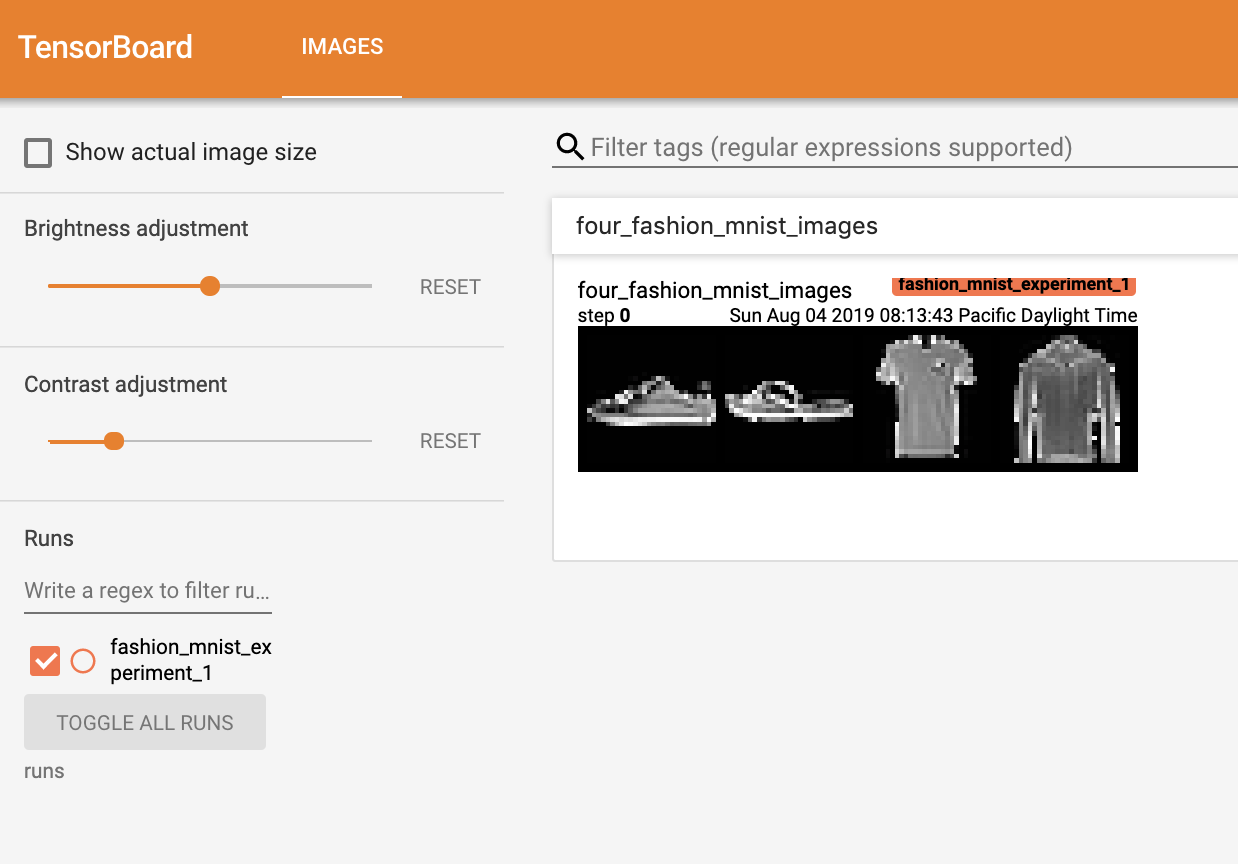
我们首先要用make_grid函数创建一个图像网格,转化为一个形状为 (B, C, H, W) 的张量,其中 B 是批次大小,C 是通道数,H 和 W 是图片的高度和宽度,再使用add_image函数写入TensorBoard
函数参数列表 :tag , img_tensor , global_step=None , walltime=None , _dataformats=’NCHW’
1 2 3 4 5 6 7 8 9 10 11 12 dataiter = iter (trainloader) images, labels = next (dataiter) img_grid = torchvision.utils.make_grid(images) matplotlib_imshow(img_grid, one_channel=True ) writer.add_image('four_fashion_mnist_images' , img_grid)
然后再命令行中输入下面命令,会输出一个http://localhost:6006 的链接,你可以直接在浏览器中打开,就能看到tensorboard中的图片
1 tensorboard --logdir=runs
查看模型结构
我们利用TensorBoardd的add_graph函数来查看一下我们上面构建的网络结构:
add_graph函数参数: model , input_to_model=None , verbose=False , use_strict_trace=True )
1
2
writer.add_graph(net, images) writer.close()
现在刷新一下浏览器页面,你们能在GRAPHS的标签栏下查看网络结构,你可以双击某个部分看到内部的结构如何实现的
数据投影可视化
我们利用add_embedding函数来对数据进行降维展示:
函数参数 mat , metadata=None , label_img=None , global_step=None , tag=’default’ , metadata_header=None )
1 2 3 4 5 6 7 8 9 10 11 12 13 14 15 16 17 18 19 20 21 22 23 24 25 26 27 28 29 30 31 32 33 34 35 36 37 38 39 def select_n_random (data, labels, n=100 ): ''' 从数据集中随机选择n个数据点及其对应的标签 参数: data: 图像数据张量 (例如: trainset.data) labels: 对应的标签张量 (例如: trainset.targets) n: 要选择的样本数量,默认为100 返回: 随机选择的n个图像和对应的n个标签 ''' assert len (data) == len (labels) perm = torch.randperm(len (data)) return data[perm][:n], labels[perm][:n] images, labels = select_n_random(trainset.data, trainset.targets) class_labels = [classes[lab] for lab in labels] features = images.view(-1 , 28 * 28 ) writer.add_embedding( features, metadata=class_labels, label_img=images.unsqueeze(1 ) ) writer.close()
现在,在TensorBoard的“PROJECTEOR”选项卡中,您可以看到这100张图片——每张图片都是784维的——被投射到三维空间中。你可以点击并拖动来旋转三维投影,并且将背景设置为黑色更容易看见。
记录模型的训练过程
1
2
3
4
5
6
7
8
9
10
11
12
13
14
15
16
17
18
19
20
21
22
23
24
25
26
27
28
29
30
31
32
33
34
35
36
37
38
39
40
41
42
43
44
45
46
47
48
49
50
51
52
53
54
55
56
57
58
59
60
61
62
63
def images_to_probs (net, images ): ''' 用训练好的网络对图像进行预测,返回预测类别和对应概率 参数: net: 训练好的神经网络模型 images: 输入图像张量 (batch_size x channels x height x width) 返回: preds: 预测的类别索引数组 probs: 每个预测对应的概率值列表 ''' output = net(images) _, preds_tensor = torch.max (output, dim=1 ) preds = np.squeeze(preds_tensor.numpy()) probs = [ F.softmax(el, dim=0 )[i].item() for i, el in zip (preds, output) ] return preds, probs def plot_classes_preds (net, images, labels ): ''' 生成显示网络预测结果的matplotlib图像 参数: net: 训练好的网络 images: 图像张量 (batch_size x channels x height x width) labels: 真实标签张量 返回: matplotlib的Figure对象 ''' preds, probs = images_to_probs(net, images) fig = plt.figure(figsize=(12 , 48 )) for idx in np.arange(4 ): ax = fig.add_subplot(1 , 4 , idx+1 , xticks=[], yticks=[]) matplotlib_imshow(images[idx], one_channel=True ) ax.set_title( "{0}, {1:.1f}%\n(label: {2})" .format ( classes[preds[idx]], probs[idx] * 100.0 , classes[labels[idx]] ), color=("green" if preds[idx]==labels[idx].item() else "red" ) ) return fig
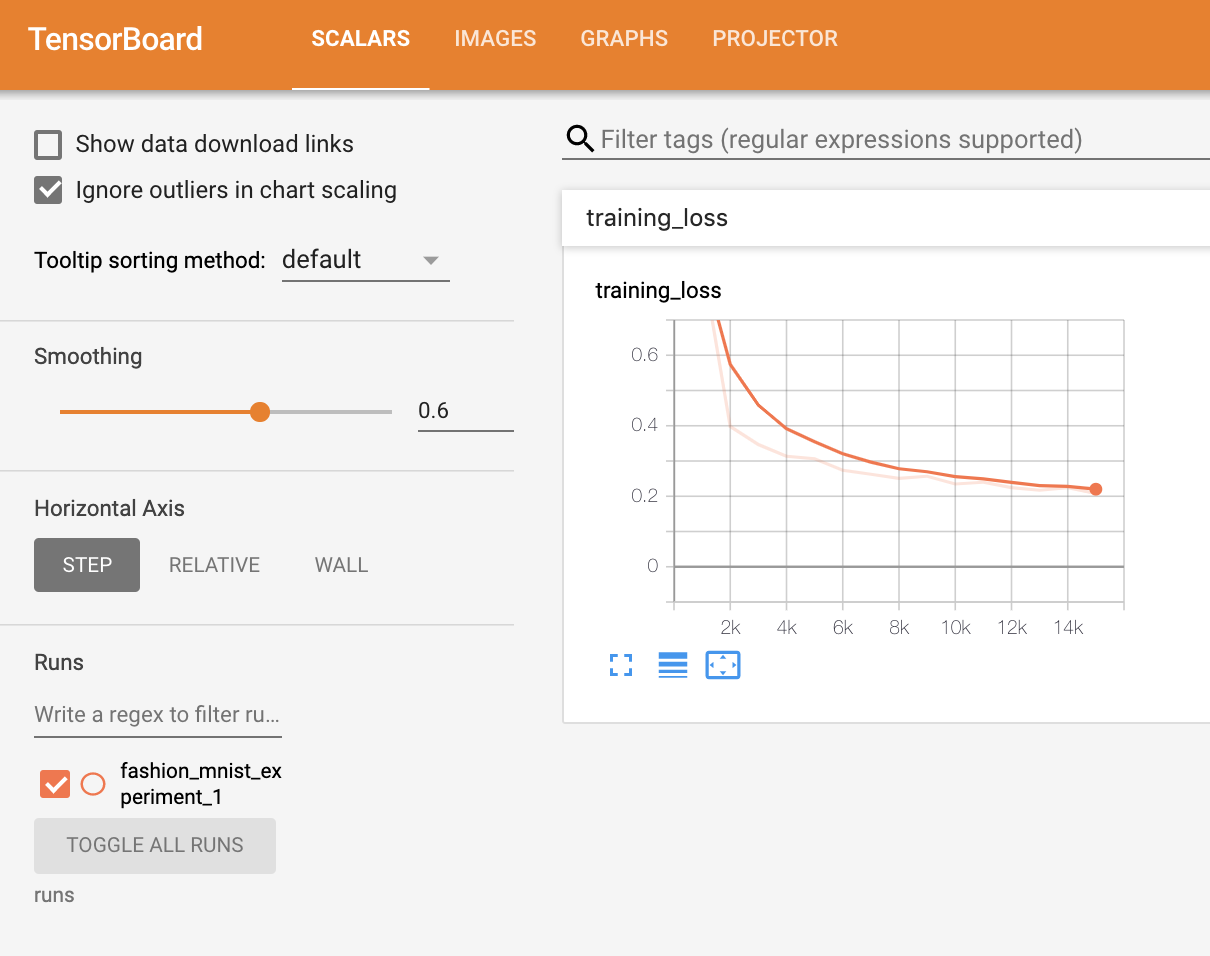
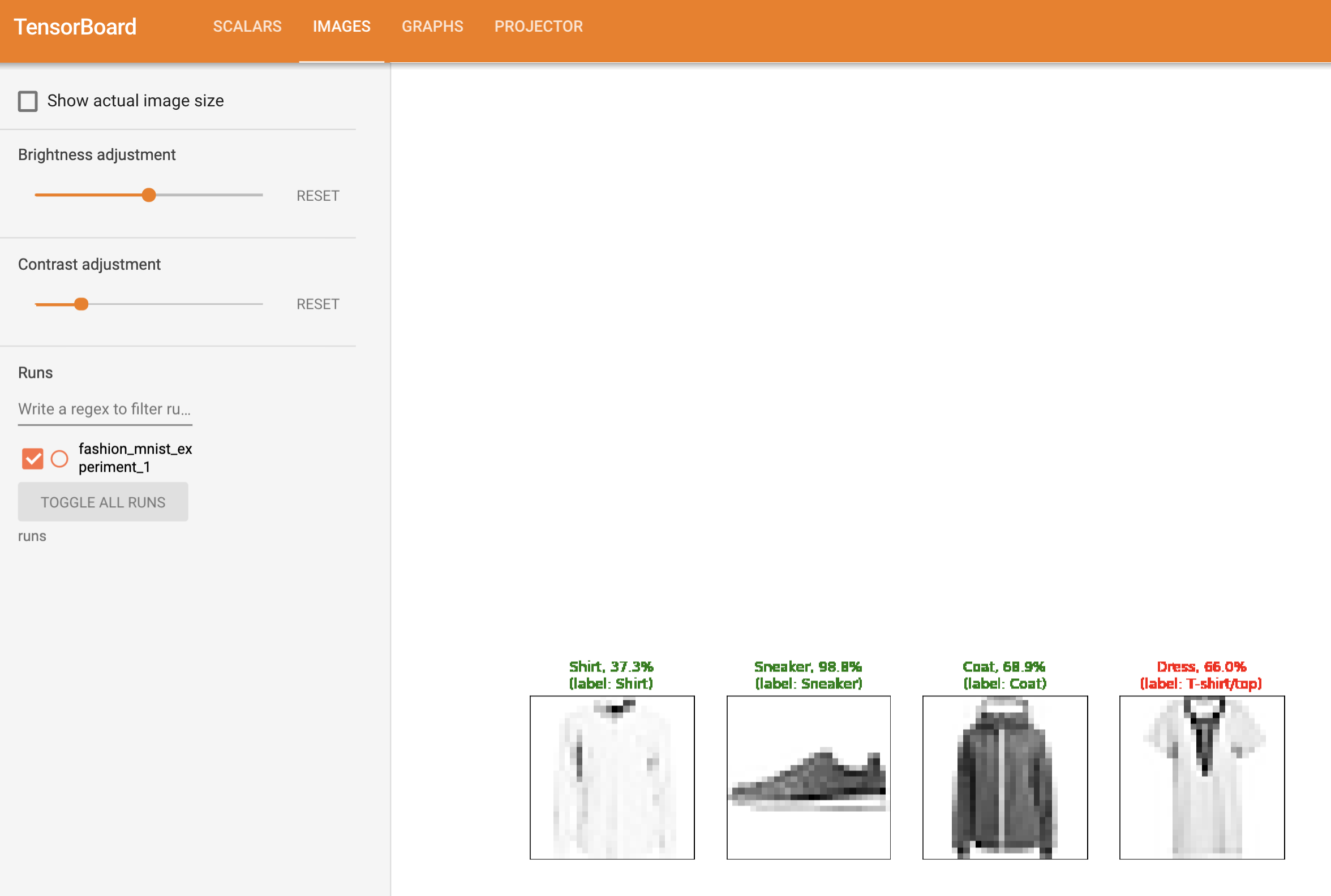
我们使用相同的模型训练代码来训练模型,每1000批次将结果写入TensorBoard,而不是打印到控制台,这是使用add_scalar函数完成的。此外,当我们训练时,我们将生成一个图像,显示模型的预测与该批次中包含的四张图片的实际结果。
add_saclar函数 tag , scalar_value , global_step=None , walltime=None , new_style=False , double_precision=False )
add_figrues函数 tag , figure , global_step=None , close=True , walltime=None
1
2
3
4
5
6
7
8
9
10
11
12
13
14
15
16
17
18
19
20
21
22
23
24
25
26
27
28
29
30
31
32
running_loss = 0.0 for epoch in range (1 ): for i, data in enumerate (trainloader, 0 ): inputs, labels = data optimizer.zero_grad() outputs = net(inputs) loss = criterion(outputs, labels) loss.backward() optimizer.step() running_loss += loss.item() if i % 1000 == 999 : writer.add_scalar('training loss' , running_loss / 1000 , epoch * len (trainloader) + i) writer.add_figure('predictions vs. actuals' , plot_classes_preds(net, inputs, labels), global_step=epoch * len (trainloader) + i) running_loss = 0.0 print ('Finished Training' )
现在你可以在浏览器中看到下面两个图片:
模型评估 例子 )。
函数参数: tag , labels , predictions , global_step=None , num_thresholds=127 , weights=None , walltime=None
1
2
3
4
5
6
7
8
9
10
11
12
13
14
15
16
17
18
19
20
21
22
23
24
25
26
27
28
29
30
31
32
33
34
35
36
37
38
39
40
41
42
43
44
45
class_probs = [] class_label = [] with torch.no_grad(): for data in testloader: images, labels = data output = net(images) class_probs_batch = [F.softmax(el, dim=0 ) for el in output] class_probs.append(class_probs_batch) class_label.append(labels) test_probs = torch.cat([torch.stack(batch) for batch in class_probs]) test_label = torch.cat(class_label) def add_pr_curve_tensorboard (class_index, test_probs, test_label, global_step=0 ): ''' 为指定类别绘制PR曲线并记录到TensorBoard 参数: class_index: 类别索引(0-9) test_probs: 所有测试样本的预测概率 [N,10] test_label: 所有测试样本的真实标签 [N] global_step: 记录步数(用于TensorBoard滑动窗口) ''' tensorboard_truth = (test_label == class_index) tensorboard_probs = test_probs[:, class_index] writer.add_pr_curve( classes[class_index], tensorboard_truth, tensorboard_probs, global_step=global_step ) for i in range (len (classes)): add_pr_curve_tensorboard(i, test_probs, test_label)
然后你就可以在浏览器中查看每个类的召回率,下面有一个例子来展示具体的计算过程:
假设我们有一个微型测试集(5个样本)和3个类别(简化计算),真实标签和预测概率如下:真实标签 (3个类别: 0,1,2)
模型预测的概率 (每个样本对3个类别的预测概率)
以类别0为例计算PR曲线
提取当前类别的相关数据
1
2
3
4
5
6
class_index = 0 tensorboard_truth = (test_label == class_index) tensorboard_probs = test_probs[:, class_index] print ("属于类别0的真实标签:" , tensorboard_truth) print ("对类别0的预测概率:" , tensorboard_probs)
按概率从高到低排序
将样本按预测概率降序排列,并对应真实标签:
1
2
3
4
5
sorted_probs, sorted_indices = torch.sort(tensorboard_probs, descending=True ) sorted_truth = tensorboard_truth[sorted_indices] print ("排序后的概率:" , sorted_probs) print ("对应的真实标签:" , sorted_truth)
动态计算Precision和Recall
逐步降低阈值,计算每个阈值下的PR值“
阈值
预测为正的样本
TP
FP
Precision
Recall
>0.8
样本1
1
0
1.0
0.5
>0.3
样本1,3
2
0
1.0
1.0
>0.2
样本1,3,2
2
1
0.67
1.0
>0.1
样本1,3,2,4,5
2
3
0.4
1.0
计算过程 :
阈值>0.8 :
阈值>0.3 :
样本1和3被预测为正
TP=2(样本1和3真实都为0),FP=0
Precision = 2/2 = 1.0
Recall = 2/2 = 1.0
阈值>0.2 :
阈值>0.1 :
所有样本被预测为正
TP=2,FP=3
Precision = 2/5 = 0.4
Recall = 2/2 = 1.0
生成PR曲线数据点
最终得到PR曲线的坐标点:
1
2
precision = [1.0 , 1.0 , 0.67 , 0.4 ] recall = [0.5 , 1.0 , 1.0 , 1.0 ]