在这个部分我们将会学习如何利用神经网络将文本进行翻译,这部分的内容具有一定的难度和深度,主要是网络结构变得更加复杂,请一定要耐心做完。
我们需要创建一个从序列到序列的神经网络,从而需要两个RNN网络来完成这件事,首先构建一个名为“Encoder”(编码器)的RNN,完成将一句话转化为一个向量,再构建一个名为“ Decoder”(解码器)的RNN,将Encoder生成的向量转化为一句话,这就是我们的工作流程。同时为了提高模型的能力,我们在此添加了注意力机制
Requirements
1
2
3
4
5
6
7
8
9
10
11
12
13
14
15
16
from __future__ import unicode_literals, print_function, divisionfrom io import open import unicodedataimport reimport randomimport torchimport torch.nn as nnfrom torch import optimimport torch.nn.functional as Fimport numpy as npfrom torch.utils.data import TensorDataset, DataLoader, RandomSampler%matplotlib inline device = torch.device("cuda" if torch.cuda.is_available() else "cpu" )
Loading data files
我们在前一部分下载的data文件夹下面有eng-fra.txt,文件里面具有英语到法语的对应字段。为了将语句输入到神经网络中,我们需要构建一个类Lang来帮助我们构建一个字典,实现word->index(word2index) and index->word(index2word),同时我们使用word2count来记录单词出现的次数
1 2 3 4 5 6 7 8 9 10 11 12 13 14 15 16 17 18 19 20 21 22 23 24 25 26 SOS_token = 0 EOS_token = 1 class Lang : def __init__ (self, name ): self .name = name self .word2index = {} self .word2count = {} self .index2word = {0 : "SOS" , 1 : "EOS" } self .n_words = 2 def addSentence (self, sentence ): for word in sentence.split(' ' ): self .addWord(word) def addWord (self, word ): if word not in self .word2index: self .word2index[word] = self .n_words self .word2count[word] = 1 self .index2word[self .n_words] = word self .n_words += 1 else : self .word2count[word] += 1
接下来是常规的进行字符处理,处理成符合ascii的字符类型,稍微看看就行
1 2 3 4 5 6 7 8 9 10 11 12 13 14 def unicodeToAscii (s ): return '' .join( c for c in unicodedata.normalize('NFD' , s) if unicodedata.category(c) != 'Mn' ) def normalizeString (s ): s = unicodeToAscii(s.lower().strip()) s = re.sub(r"([.!?])" , r" \1" , s) s = re.sub(r"[^a-zA-Z!?]+" , r" " , s) return s.strip()
从文件读取两种语言,并用一个reverse标志符号确实是从哪个语言翻译为另一个语言,代码很简单,相信大家都能看懂:
1
2
3
4
5
6
7
8
9
10
11
12
13
14
15
16
17
18
19
20
21
def readLangs (lang1, lang2, reverse=False ): """读取双语文本文件,处理并返回语言对象和句子对""" print ("Reading lines..." ) lines = open ('data/%s-%s.txt' % (lang1, lang2), encoding='utf-8' ).read().strip().split('\n' ) pairs = [[normalizeString(s) for s in l.split('\t' )] for l in lines] if reverse: pairs = [list (reversed (p)) for p in pairs] input_lang = Lang(lang2) output_lang = Lang(lang1) else : input_lang = Lang(lang1) output_lang = Lang(lang2) return input_lang, output_lang, pairs
语句的长度大多数是长短不一样的,在这里我们为了让模型训练速度更快,使用最大长度为10个单词的语句,同时英语语句的开头必须符合主谓结构
1
2
3
4
5
6
7
8
9
10
11
12
13
14
15
16
17
18
19
20
MAX_LENGTH = 10 eng_prefixes = ( "i am " , "i m " , "he is" , "he s " , "she is" , "she s " , "you are" , "you re " , "we are" , "we re " , "they are" , "they re " ) def filterPair (p ): return len (p[0 ].split(' ' )) < MAX_LENGTH and \ len (p[1 ].split(' ' )) < MAX_LENGTH and \ p[1 ].startswith(eng_prefixes) def filterPairs (pairs ): return [pair for pair in pairs if filterPair(pair)]
数据准备的过程:
读取文件并且将文本内容转化为句子对(pairs)
规范化文本,按长度和开头语句过滤
用句子对形成 word list
1
2
3
4
5
6
7
8
9
10
11
12
13
14
15
16
17
18
19
20
21
22
23
24
25
26
def prepareData (lang1, lang2, reverse=False ): """准备训练数据:读取数据、过滤句子对、构建词汇表""" input_lang, output_lang, pairs = readLangs(lang1, lang2, reverse) print ("Read %s sentence pairs" % len (pairs)) pairs = filterPairs(pairs) print ("Trimmed to %s sentence pairs" % len (pairs)) print ("Counting words..." ) for pair in pairs: input_lang.addSentence(pair[0 ]) output_lang.addSentence(pair[1 ]) print ("Counted words:" ) print (input_lang.name, input_lang.n_words) print (output_lang.name, output_lang.n_words) return input_lang, output_lang, pairs input_lang, output_lang, pairs = prepareData('eng' , 'fra' , True ) print (random.choice(pairs))
The Seq2Seq Model
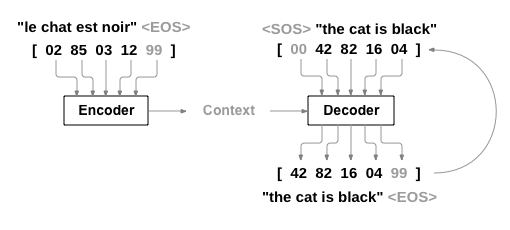
RNN是一个在序列上运行并使用自己的输出作为后续步骤的输入的网络;seq2seq网络 ,或编码器解码器网络 ,是一个由两个RNN组成的模型,称为编码器和解码器。编码器读取输入序列并输出单个向量,解码器读取该向量以产生输出序列。
与单个RNN的序列预测不同,每个输入都对应一个输出,seq2seq模型将我们从序列长度和顺序中解放出来,这使得它非常适合两种语言之间的翻译。
考虑句子Je ne suis pas le chat noir → I am not the black cat输入句子中的大多数单词在输出句子中有直接翻译,但顺序略有不同,例如chat noir 和 black cat。由于ne/pas结构,输入句子中还有一个单词。很难直接从输入的单词序列中产生正确的翻译。
使用seq2seq模型,编码器创建了一个单一向量,在理想情况下,该向量将输入序列的“含义”编码为单个向量——一些N维句子空间中的单点。模型的结构如下
The Encoder
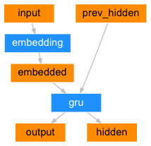
编码器的结构如图所示:
构建一个Encoder类,其中 embedding 层是用于将单词的索引转化成一个连续的向量(思考为什么不是转化为 one-hot 向量),gru 层是 RNN 网络的一种变体,dropout 层用来防止过拟合;正向传播的过程可以结合图示更加清晰。
1
2
3
4
5
6
7
8
9
10
11
12
13
class EncoderRNN (nn.Module): def __init__ (self, input_size, hidden_size, dropout_p=0.1 ): super (EncoderRNN, self ).__init__() self .hidden_size = hidden_size self .embedding = nn.Embedding(input_size, hidden_size) self .gru = nn.GRU(hidden_size, hidden_size, batch_first=True ) self .dropout = nn.Dropout(dropout_p) def forward (self, input ): embedded = self .dropout(self .embedding(input )) output, hidden = self .gru(embedded) return output, hidden
The Decoder
Simple Decoder
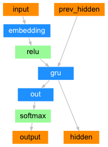
在最简单的seq2seq解码器中,我们只使用编码器的最后一个输出。最后一个输出有时被称为上下文向量(context vector),因为它对整个序列的上下文进行编码。此上下文向量用作解码器的初始隐藏状态。
在解码的每个步骤中,解码器都会得到一个输入令牌和隐藏状态。初始输入令牌是字符串开头<SOS>令牌,第一个隐藏状态是上下文向量,同样是编码器的最后一个隐藏状态,这也是为什么两个网络能够结合起来发挥能力的重要原因。结构如图:
同样我们在解码器中定义了 embeddind 层,gru 层。前向传播过程中的代码稍微多一点,因为一个句子会有很多单词,而我们需要单词一个一个的预测。我们添加了target_tensor参数,主要作用是在训练的过程中,我们将真实的单词作为下一个输入,而在测试的时候我们将当前预测的单词作为下一个输入。前向传播的过程是我们从编码器获得隐藏状态,然后在循环中进行当前单词的预测,循环结构将每一步预测的单词拼接起来。
1
2
3
4
5
6
7
8
9
10
11
12
13
14
15
16
17
18
19
20
21
22
23
24
25
26
27
28
29
30
31
32
33
34
35
36
37
38
39
40
41
42
43
44
45
46
47
48
49
50
51
52
53
54
55
56
57
58
class DecoderRNN (nn.Module): """基于GRU的RNN解码器,用于序列生成任务(如机器翻译)""" def __init__ (self, hidden_size, output_size ): """ 初始化解码器 :param hidden_size: 隐藏层维度(与编码器保持一致) :param output_size: 输出词汇表大小(目标语言词表大小) """ super (DecoderRNN, self ).__init__() self .embedding = nn.Embedding(output_size, hidden_size) self .gru = nn.GRU(hidden_size, hidden_size, batch_first=True ) self .out = nn.Linear(hidden_size, output_size) def forward (self, encoder_outputs, encoder_hidden, target_tensor=None ): """ 前向传播(生成目标序列) :param encoder_outputs: 编码器输出(通常未直接使用) :param encoder_hidden: 编码器的最终隐藏状态(作为解码器初始状态) :param target_tensor: 目标序列(用于Teacher Forcing训练模式) :return: (输出序列概率, 最终隐藏状态, None) """ batch_size = encoder_outputs.size(0 ) decoder_input = torch.empty(batch_size, 1 , dtype=torch.long, device=device).fill_(SOS_token) decoder_hidden = encoder_hidden decoder_outputs = [] for i in range (MAX_LENGTH): decoder_output, decoder_hidden = self .forward_step(decoder_input, decoder_hidden) decoder_outputs.append(decoder_output) if target_tensor is not None : decoder_input = target_tensor[:, i].unsqueeze(1 ) else : _, topi = decoder_output.topk(1 ) decoder_input = topi.squeeze(-1 ).detach() decoder_outputs = torch.cat(decoder_outputs, dim=1 ) decoder_outputs = F.log_softmax(decoder_outputs, dim=-1 ) return decoder_outputs, decoder_hidden, None def forward_step (self, input , hidden ): """单步解码过程""" output = self .embedding(input ) output = F.relu(output) output, hidden = self .gru(output, hidden) output = self .out(output) return output, hidden
Attention Decoder
如果只有上下文向量在编码器和解码器之间传递,则该单个向量承担了编码整个句子的负担。
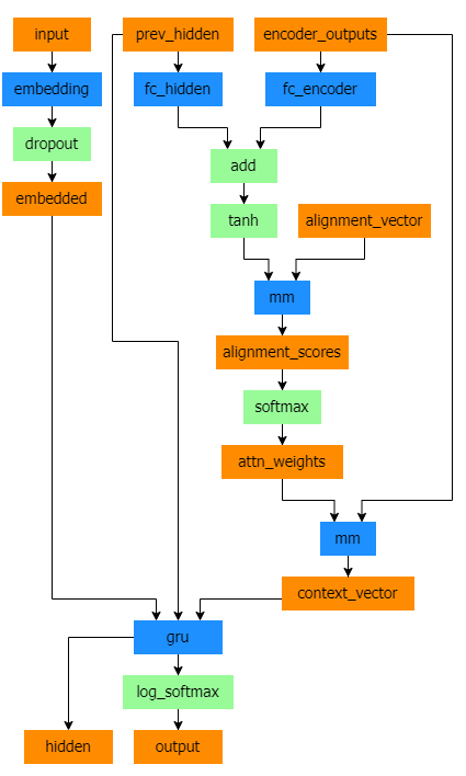
注意力机制允许解码器网络在解码器自身输出的每个步骤中“专注于”编码器输出的不同部分。首先,我们计算一组注意力权重。这些将乘以编码器输出向量,以创建一个加权组合。结果(在代码中称为attn_applied)应包含有关输入序列特定部分的信息,从而帮助解码器选择正确的输出词。计算注意力权重是用另一个前馈层 attn 完成的,使用解码器的输入和隐藏状态作为输入。由于训练数据中包含各种大小的句子,为了实际创建和训练此层,我们必须选择可以应用的最大句子长度(输入长度,用于编码器输出)。最大长度的句子将使用所有注意力权重,而较短的句子将只使用前几个。解码器的结构如下图:
Bahdanau注意力,也称为 additive attention,是 Sqe2Sqe 模型中常用的注意力机制,特别是在神经机器翻译任务中。这种注意力机制采用学习的对齐模型来计算编码器和解码器隐藏状态之间的注意力分数。它利用前馈神经网络来计算对齐分数。
然而,还有可用的替代注意力机制,例如Luong注意力,它通过在解码器隐藏状态和编码器隐藏状态之间取得分来计算注意力分数。它不涉及Bahdanau注意力中使用的非线性变换。
在本教程中,我们将使用Bahdanau的注意力。然而,探索修改注意力机制以使用Luong注意力将是一项有价值的练习。
在Bahdanau注意力机制中我们定义了三个线性变换层:
线性层
输入
输出
功能说明
Wa解码器的当前隐藏状态 (query)
[batch_size, 1, hidden_size]将解码器的隐藏状态映射到一个新的空间,用于与编码器输出计算匹配度
Ua编码器的所有输出 (keys)
[batch_size, seq_len, hidden_size]将编码器的每个时间步输出映射到与Wa(query)相同的空间,便于计算交互作用
Va加和后的中间结果
[batch_size, seq_len, 1]将交互结果压缩为一个标量分数(注意力分数),再通过softmax归一化为权重
前向传播过程:
Wa(query)query)经过线性变换,维度不变,但映射到与编码器输出对齐的空间。Ua(keys)keys)分别经过线性变换,维度不变,但映射到与解码器状态对齐的空间。相加 + tanh
将Wa(query)广播(复制)到与Ua(keys)相同的序列长度,然后逐元素相加。
通过tanh激活函数引入非线性,增强表达能力。
Va 计算分数Va映射为一个标量分数(即注意力分数),表示解码器当前步对编码器某位置的关注程度。
在注意力解码器中,在保留其他层的条件下,我们将上述构建的BahdanauAttention 添加到网络中。在前向传播中整体与非注意力机制的传播过程相同,多了一个attention参数,更重要的是在 单步前向传播过程中的计算:forward_step 方法是带有注意力机制的RNN解码器的核心操作,它定义了解码器单步生成 的过程。下面我将逐步解析每一部分的实现和作用:
1. 输入嵌入 (Input Embedding)
1 embedded = self .dropout(self .embedding(input ))
输入 :input 是当前时间步的解码器输入(单词索引),形状为 [batch_size, 1] 处理 :
self.embedding:将单词索引转换为稠密向量([batch_size, 1, hidden_size])self.dropout:随机屏蔽部分神经元,防止过拟合(训练时生效)
输出 :embedded 是当前词的嵌入表示,形状 [batch_size, 1, hidden_size]
2. 注意力计算 (Attention Mechanism)
1
2
query = hidden.permute(1 , 0 , 2 ) context, attn_weights = self .attention(query, encoder_outputs)
query 调整
hidden 是解码器上一时间步的隐藏状态,原始形状为 [num_layers, batch_size, hidden_size](GRU的默认输出格式) permute(1, 0, 2) 将其调整为 [batch_size, 1, hidden_size] 以匹配注意力层的输入要求
注意力计算 :
self.attention(query, encoder_outputs) 调用 BahdanauAttention,返回:
context:上下文向量(编码器输出的加权和),形状 [batch_size, 1, hidden_size] attn_weights:注意力权重(概率分布),形状 [batch_size, 1, src_seq_len]
3. GRU 输入准备
1 input_gru = torch.cat((embedded, context), dim=2 )
拼接操作 :embedded 和注意力生成的上下文向量 context 在特征维度(dim=2)拼接 输出形状 :[batch_size, 1, 2 * hidden_size] 意义 :
当前词的语义(embedded)
源序列中与当前步最相关的上下文信息(context)
4. GRU 处理和输出预测
1
2
output, hidden = self .gru(input_gru, hidden) output = self .out(output)
GRU 处理 :
输入:拼接后的 input_gru 和上一时间步的 hidden 状态
输出:
output:当前时间步的GRU输出,形状 [batch_size, 1, hidden_size] hidden:更新后的隐藏状态(传递给下一步),形状 [num_layers, batch_size, hidden_size]
线性变换 :self.out 将 output 映射到目标词表空间,形状变为 [batch_size, 1, output_size](output_size 是目标词汇表大小)
5. 返回值
1 return output, hidden, attn_weights
outputhiddenattn_weights
1
2
3
4
5
6
7
8
9
10
11
12
13
14
15
16
17
18
19
20
21
22
23
24
25
26
27
28
29
30
31
32
33
34
35
36
37
38
39
40
41
42
43
44
45
46
47
48
49
50
51
52
53
54
55
56
57
58
59
60
61
62
63
64
65
66
67
68
69
70
71
72
73
74
75
76
77
78
79
80
81
82
83
84
85
86
87
88
89
90
91
92
93
94
95
96
97
98
99
100
101
102
103
class BahdanauAttention (nn.Module): """Bahdanau注意力机制(加性注意力)""" def __init__ (self, hidden_size ): """ 初始化注意力层 :param hidden_size: 隐藏层维度(必须与编码器/解码器保持一致) """ super (BahdanauAttention, self ).__init__() self .Wa = nn.Linear(hidden_size, hidden_size) self .Ua = nn.Linear(hidden_size, hidden_size) self .Va = nn.Linear(hidden_size, 1 ) def forward (self, query, keys ): """ 计算注意力上下文向量 :param query: 解码器当前隐藏状态 [batch_size, 1, hidden_size] :param keys: 编码器所有输出 [batch_size, seq_len, hidden_size] :return: (上下文向量, 注意力权重) """ scores = self .Va(torch.tanh(self .Wa(query) + self .Ua(keys))) scores = scores.squeeze(2 ).unsqueeze(1 ) weights = F.softmax(scores, dim=-1 ) context = torch.bmm(weights, keys) return context, weights class AttnDecoderRNN (nn.Module): """带注意力机制的RNN解码器""" def __init__ (self, hidden_size, output_size, dropout_p=0.1 ): """ 初始化解码器 :param hidden_size: 隐藏层维度 :param output_size: 输出词表大小 :param dropout_p: dropout概率 """ super (AttnDecoderRNN, self ).__init__() self .embedding = nn.Embedding(output_size, hidden_size) self .attention = BahdanauAttention(hidden_size) self .gru = nn.GRU(2 * hidden_size, hidden_size, batch_first=True ) self .out = nn.Linear(hidden_size, output_size) self .dropout = nn.Dropout(dropout_p) def forward (self, encoder_outputs, encoder_hidden, target_tensor=None ): """ 前向传播(带注意力机制的序列生成) :param encoder_outputs: 编码器所有输出 [batch_size, seq_len, hidden_size] :param encoder_hidden: 编码器最终隐藏状态 [num_layers, batch_size, hidden_size] :param target_tensor: 目标序列(用于Teacher Forcing) :return: (输出序列概率, 最终隐藏状态, 注意力权重矩阵) """ batch_size = encoder_outputs.size(0 ) decoder_input = torch.empty(batch_size, 1 , dtype=torch.long, device=device).fill_(SOS_token) decoder_hidden = encoder_hidden decoder_outputs = [] attentions = [] for i in range (MAX_LENGTH): decoder_output, decoder_hidden, attn_weights = self .forward_step( decoder_input, decoder_hidden, encoder_outputs ) decoder_outputs.append(decoder_output) attentions.append(attn_weights) if target_tensor is not None : decoder_input = target_tensor[:, i].unsqueeze(1 ) else : _, topi = decoder_output.topk(1 ) decoder_input = topi.squeeze(-1 ).detach() decoder_outputs = torch.cat(decoder_outputs, dim=1 ) decoder_outputs = F.log_softmax(decoder_outputs, dim=-1 ) attentions = torch.cat(attentions, dim=1 ) return decoder_outputs, decoder_hidden, attentions def forward_step (self, input , hidden, encoder_outputs ): """单步解码过程""" embedded = self .dropout(self .embedding(input )) query = hidden.permute(1 , 0 , 2 ) context, attn_weights = self .attention(query, encoder_outputs) input_gru = torch.cat((embedded, context), dim=2 ) output, hidden = self .gru(input_gru, hidden) output = self .out(output) return output, hidden, attn_weights
Training
训练时,我们需要将所有输入变为tensor类型
1
2
3
4
5
6
7
8
9
10
11
12
13
14
15
16
17
18
19
20
21
22
23
24
25
26
27
28
29
30
31
32
33
34
35
36
37
38
39
40
41
42
43
44
45
46
47
48
49
50
51
52
53
54
def indexesFromSentence (lang, sentence ): """将句子中的每个单词转换为对应的索引列表""" return [lang.word2index[word] for word in sentence.split(' ' )] def tensorFromSentence (lang, sentence ): """将句子转换为张量形式,并添加EOS结束标记""" indexes = indexesFromSentence(lang, sentence) indexes.append(EOS_token) return torch.tensor(indexes, dtype=torch.long, device=device).view(1 , -1 ) def tensorsFromPair (pair ): """将语言对(输入句子,目标句子)转换为输入和目标张量""" input_tensor = tensorFromSentence(input_lang, pair[0 ]) target_tensor = tensorFromSentence(output_lang, pair[1 ]) return (input_tensor, target_tensor) def get_dataloader (batch_size ): """创建数据加载器(DataLoader)用于批量训练""" input_lang, output_lang, pairs = prepareData('eng' , 'fra' , True ) n = len (pairs) input_ids = np.zeros((n, MAX_LENGTH), dtype=np.int32) target_ids = np.zeros((n, MAX_LENGTH), dtype=np.int32) for idx, (inp, tgt) in enumerate (pairs): inp_ids = indexesFromSentence(input_lang, inp) inp_ids.append(EOS_token) input_ids[idx, :len (inp_ids)] = inp_ids tgt_ids = indexesFromSentence(output_lang, tgt) tgt_ids.append(EOS_token) target_ids[idx, :len (tgt_ids)] = tgt_ids train_data = TensorDataset( torch.LongTensor(input_ids).to(device), torch.LongTensor(target_ids).to(device) ) train_sampler = RandomSampler(train_data) train_dataloader = DataLoader( train_data, sampler=train_sampler, batch_size=batch_size ) return input_lang, output_lang, train_dataloader
Training the Model
为了训练,我们通过编码器运行输入句子,并跟踪每个输出和最新的隐藏状态。然后,解码器被赋予<SOS>令牌作为其第一个输入,编码器的最后一个隐藏状态作为其第一个隐藏状态。
“Teacher Forcing”是指使用实际目标输出作为下一个输入,而不是使用解码器的猜测作为下一个输入的概念。使用Teacher Forcing会导致它收敛得更快,但当训练有素的网络被利用时,它可能会表现出不稳定。
你可以观察Teacher Forcing网络的输出,这些网络用连贯的语法阅读,但远离正确的翻译——直观地,它已经学会了表示输出语法,一旦teacher告诉它前几个单词,就可以理解意思,但它一开始就没有正确学会如何从翻译中创建句子。
这部分内容和之前的差不多,因此不再赘述。
1
2
3
4
5
6
7
8
9
10
11
12
13
14
15
16
17
18
19
20
21
22
23
24
25
def train_epoch (dataloader, encoder, decoder, encoder_optimizer, decoder_optimizer, criterion ): total_loss = 0 for data in dataloader: input_tensor, target_tensor = data encoder_optimizer.zero_grad() decoder_optimizer.zero_grad() encoder_outputs, encoder_hidden = encoder(input_tensor) decoder_outputs, _, _ = decoder(encoder_outputs, encoder_hidden, target_tensor) loss = criterion( decoder_outputs.view(-1 , decoder_outputs.size(-1 )), target_tensor.view(-1 ) ) loss.backward() encoder_optimizer.step() decoder_optimizer.step() total_loss += loss.item() return total_loss / len (dataloader)
我们添加一个运行时间的函数
1
2
3
4
5
6
7
8
9
10
11
12
13
14
import timeimport mathdef asMinutes (s ): m = math.floor(s / 60 ) s -= m * 60 return '%dm %ds' % (m, s) def timeSince (since, percent ): now = time.time() s = now - since es = s / (percent) rs = es - s return '%s (- %s)' % (asMinutes(s), asMinutes(rs))
整个流程的训练代码如下:
1
2
3
4
5
6
7
8
9
10
11
12
13
14
15
16
17
18
19
20
21
22
23
24
25
26
27
28
def train (train_dataloader, encoder, decoder, n_epochs, learning_rate=0.001 , print_every=100 , plot_every=100 ): start = time.time() plot_losses = [] print_loss_total = 0 plot_loss_total = 0 encoder_optimizer = optim.Adam(encoder.parameters(), lr=learning_rate) decoder_optimizer = optim.Adam(decoder.parameters(), lr=learning_rate) criterion = nn.NLLLoss() for epoch in range (1 , n_epochs + 1 ): loss = train_epoch(train_dataloader, encoder, decoder, encoder_optimizer, decoder_optimizer, criterion) print_loss_total += loss plot_loss_total += loss if epoch % print_every == 0 : print_loss_avg = print_loss_total / print_every print_loss_total = 0 print ('%s (%d %d%%) %.4f' % (timeSince(start, epoch / n_epochs), epoch, epoch / n_epochs * 100 , print_loss_avg)) if epoch % plot_every == 0 : plot_loss_avg = plot_loss_total / plot_every plot_losses.append(plot_loss_avg) plot_loss_total = 0 showPlot(plot_losses)
结果绘制:
1
2
3
4
5
6
7
8
9
10
11
12
import matplotlib.pyplot as pltplt.switch_backend('agg' ) import matplotlib.ticker as tickerimport numpy as npdef showPlot (points ): plt.figure() fig, ax = plt.subplots() loc = ticker.MultipleLocator(base=0.2 ) ax.yaxis.set_major_locator(loc) plt.plot(points)
Evaluation
1
2
3
4
5
6
7
8
9
10
11
12
13
14
15
16
17
18
19
20
21
22
23
24
25
26
27
def evaluate (encoder, decoder, sentence, input_lang, output_lang ): with torch.no_grad(): input_tensor = tensorFromSentence(input_lang, sentence) encoder_outputs, encoder_hidden = encoder(input_tensor) decoder_outputs, decoder_hidden, decoder_attn = decoder(encoder_outputs, encoder_hidden) _, topi = decoder_outputs.topk(1 ) decoded_ids = topi.squeeze() decoded_words = [] for idx in decoded_ids: if idx.item() == EOS_token: decoded_words.append('<EOS>' ) break decoded_words.append(output_lang.index2word[idx.item()]) return decoded_words, decoder_attn def evaluateRandomly (encoder, decoder, n=10 ): for i in range (n): pair = random.choice(pairs) print ('>' , pair[0 ]) print ('=' , pair[1 ]) output_words, _ = evaluate(encoder, decoder, pair[0 ], input_lang, output_lang) output_sentence = ' ' .join(output_words) print ('<' , output_sentence) print ('' )
End: Training and Evaluating
1
2
3
4
5
6
7
8
9
hidden_size = 128 batch_size = 32 input_lang, output_lang, train_dataloader = get_dataloader(batch_size) encoder = EncoderRNN(input_lang.n_words, hidden_size).to(device) decoder = AttnDecoderRNN(hidden_size, output_lang.n_words).to(device) train(train_dataloader, encoder, decoder, 80 , print_every=5 , plot_every=5 )
1 2 3 encoder.eval () decoder.eval () evaluateRandomly(encoder,decoder)
Visualizing Attention
我们通过一个热力图来使得注意力机制可视化
这个函数用于绘制注意力权重图。
参数 :
input_sentence: 输入的源语言句子(法语)output_words: 模型输出的目标语言单词(英语)attentions: 注意力权重矩阵
功能 :
创建一个热力图显示注意力权重
设置x轴为输入句子的单词(加上<EOS>结束符)
设置y轴为输出单词
确保每个刻度都显示标签
显示图形
这个函数结合了评估和可视化功能。
参数 :
功能 :
调用evaluate函数获取翻译结果和注意力权重
打印输入和输出句子
调用showAttention显示注意力权重图
1
2
3
4
5
6
7
8
9
10
11
12
13
14
15
16
17
18
19
20
21
22
23
24
25
26
27
28
29
30
31
32
33
def showAttention (input_sentence, output_words, attentions ): fig = plt.figure() ax = fig.add_subplot(111 ) cax = ax.matshow(attentions.cpu().numpy(), cmap='bone' ) fig.colorbar(cax) x_labels = ['' ] + input_sentence.split(' ' ) + ['<EOS>' ] ax.set_xticks(range (len (x_labels))) ax.set_xticklabels(x_labels, rotation=90 ) y_labels = ['' ] + output_words ax.set_yticks(range (len (y_labels))) ax.set_yticklabels(y_labels) plt.show() def evaluateAndShowAttention (input_sentence ): output_words, attentions = evaluate(encoder, decoder, input_sentence,input_lang, output_lang) print ('input = ' , input_sentence) print ('output = ' ,' ' .join(output_words)) showAttention(input_sentence,output_words,attentions[0 ,:len (output_words),:]) evaluateAndShowAttention('il n est pas aussi grand que son pere' ) evaluateAndShowAttention('je suis trop fatigue pour conduire' ) evaluateAndShowAttention('je suis desole si c est une question idiote' ) evaluateAndShowAttention('je suis reellement fiere de vous' )
More
Related Paper
Learning Phrase Representations using RNN Encoder-Decoder for Statistical Machine Translation Sequence to Sequence Learning with Neural Networks Neural Machine Translation by Jointly Learning to Align and Translate A Neural Conversational Model Effective Approaches to Attention-based Neural Machine Translation.